Generating Myelin Indices Maps using Magnetization Transfer Imaging (MTI)
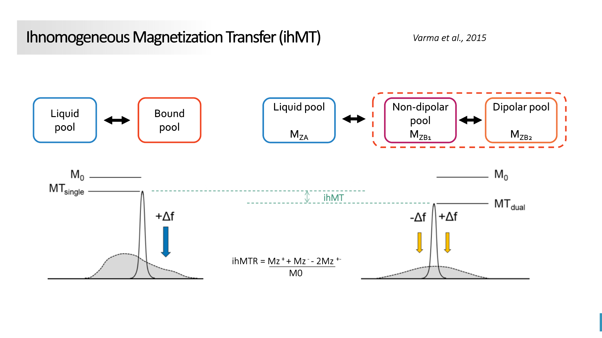
Magnetization Transfer (MT) imaging is an MRI technique that measures interactions between :
Bound protons (associated with macromolecules like myelin)
Free water protons (aqueous pool)
When saturation pulses are applied at off-resonance frequencies, the MRI signal from bound protons decreases. This attenuation depends on the macromolecular content of tissue, making MT imaging sensitive to myelin content. The inhomogeneous Magnetization Transfer (ihMT) enhances this effect by using alternating positive and negative frequency saturation pulses, improving specificity to myelin.
Play the video for more details on how MT sequence acquisition and parameter calculation work (link will be added soon) .. ToDo: Add video on YouTube (MT_WhatIsIt.mp4)
Understanding the output
The scil_mti_maps_ihMT script computes four myelin indices maps from Magnetization Transfer (MT) and inhomogeneous Magnetization Transfer (ihMT) images. These maps provide valuable information about myelin content in brain white matter.
Magnetization Transfer maps
MTR: Magnetization Transfer Ratio |
MTsat: Magnetization Transfer Saturation |
|---|---|
|
|
Inhomogeneous Magnetization Transfer maps
ihMTR: Inhomogeneous Magnetization Transfer Ratio |
ihMTsat: Inhomogeneous Magnetization Transfer Saturation |
|---|---|
|
|
Understanding the input
Acquisition Parameters
To compute MTsat and ihMTsat, acquisition parameters are required. They can be provided in two ways:
Option A – From JSON files:
–in_jsons path/to/mtoffPD.json path/to/mtoffT1.json
Option B – Manual entry:
–in_acq_parameters PD_flipAngle T1_flipAngle PD_TR T1_TR
Flip angles (in degrees)
Repetition times (in seconds)
Preparing data for this tutorial
To run lines below, you need a various volumes. The tutorial data is still in preparation, meanwhile you can use this: `
in_dir=where/you/downloaded/tutorial/data

# For now, let's use data in .scilpy
scil_data_download -v ERROR
in_dir=$in_dir/mti
mkdir $in_dir
cp $HOME/.scilpy/ihMT/B1* $in_dir/
cp $HOME/.scilpy/ihMT/echo-1* $in_dir/
cp $HOME/.scilpy/ihMT/mask_resample.nii.gz $in_dir/mask.nii.gz
These files include:
altnp – dual alternating negative/positive frequency images
altpn – dual alternating positive/negative frequency images
negative – single negative frequency images
positive – single positive frequency images
mtoff_PD – proton density unsaturated reference
mtoff_T1 (optional) – T1-weighted unsaturated reference (required for saturation maps)
Overall, we have data for a subject, containing:
├── B1map.json
├── B1map.nii.gz
├── echo-1_acq-altnp_ihmt.json
├── echo-1_acq-altnp_ihmt.nii.gz
├── echo-1_acq-altpn_ihmt.json
├── echo-1_acq-altpn_ihmt.nii.gz
├── echo-1_acq-mtoff_ihmt.json
├── echo-1_acq-mtoff_ihmt.nii.gz
├── echo-1_acq-neg_ihmt.json
├── echo-1_acq-neg_ihmt.nii.gz
├── echo-1_acq-pos_ihmt.json
├── echo-1_acq-pos_ihmt.nii.gz
├── echo-1_acq-T1w_ihmt.json    (optional)
├── echo-1_acq-T1w_ihmt.nii.gz  (optional)
└── mask.nii.gz
Tip
You may download the complete bash script to run the whole tutorial in one step ⭳ here.
Step-by-step processing
Basic Usage
Minimal command example:
scil_mti_maps_ihMT $out_dir \
    --in_altnp $in_dir/*altnp*.nii.gz \
    --in_altpn $in_dir/*altpn*.nii.gz \
    --in_negative $in_dir/*neg*.nii.gz \
    --in_positive $in_dir/echo*pos*.nii.gz \
    --in_mtoff_pd $in_dir/echo*mtoff*.nii.gz \
    --in_mtoff_t1 $in_dir/echo*T1w*.nii.gz \
    --mask $in_dir/mask.nii.gz \
    --in_jsons $in_dir/echo*mtoff*.json $in_dir/echo*T1w*.json
Replace
*with the echo index if you want a specific echo instead of all echoes.A binary mask must be aligned with all images.
Output maps are saved in
output_directory/ihMT_native_maps/.Use
--out_prefixto add a custom prefix to all output files.
Note
In the event that multiple echoes have been acquired : All contrasts must have the same number of echoes and be coregistered.
The script generates two main folders:
ihMT_native_maps/
MTR.nii.gz– Magnetization Transfer (MT) RatioihMTR.nii.gz– Inhomogeneous Magnetization Transfer RatioMTsat.nii.gz– MT saturation (if mtoff_T1 as available)ihMTsat.nii.gz– ihMT saturation (if mtoff_T1 available)
Complementary_maps/ (if ``–extended`` is set, see below)
altnp.nii.gz,altpn.nii.gz,positive.nii.gz,negative.nii.gzmtoff_PD.nii.gz,mtoff_T1.nii.gzDerived maps:
MTsat_d.nii.gz,MTsat_sp.nii.gz,MTsat_sn.nii.gz,R1app.nii.gz,B1_map.nii.gz
Similar Script: scil_mti_maps_MT
For datasets where only MT images are available (without ihMT dual alternating contrasts), a simplified script is provided:
scil_mti_maps_MT.
This script computes two myelin maps:
MTR.nii.gz – Magnetization Transfer Ratio map
MTsat.nii.gz – Magnetization Transfer saturation map
Optional outputs are available in a Complementary_maps folder, such as the individual positive/negative frequency images, unsaturated PD/T1 images, and intermediate MTsat computations.
scil_mti_maps_MT $out_dir \
    --in_positive $in_dir/echo*pos*.nii.gz \
    --in_negative $in_dir/echo*neg*.nii.gz \
    --in_mtoff_pd $in_dir/echo*mtoff*.nii.gz \
    --in_mtoff_t1 $in_dir/echo*T1w*.nii.gz \
    --mask $in_dir/mask.nii.gz \
    --in_jsons $in_dir/echo*mtoff*.json $in_dir/echo*T1w*.json
By default, all echoes are used. To use only one, replace * with the echo number.
B1 Correction
Like the ihMT script, scil_mti_maps_MT supports B1+ field inhomogeneity correction, either empiric or model-based, using the options:
--in_B1_mapto provide a B1 map--B1_correction_method empiricormodel_based--B1_fitvaluesto provide external calibration files (1 or 2 .mat files)
When to use each script
Use ``scil_mti_maps_ihMT`` if you have ihMT acquisitions (dual alternating contrasts, positive, negative, PD, T1). Produces 4 myelin maps.
Use ``scil_mti_maps_MT`` if you only have MT acquisitions (positive, negative, PD, T1). Produces 2 myelin maps.
Both scripts require coregistered inputs.
To go further
B1+ Field Correction (Optional)
The script allows correction for B1 inhomogeneity.
Empiric method:
–in_B1_map path/to/B1map.nii.gz –B1_correction_method empiric
Model-based method:
–in_B1_map path/to/B1map.nii.gz –B1_correction_method model_based –B1_fitvalues pos_fit.mat neg_fit.mat dual_fit.mat –B1_nominal 100
Note
Requires .mat files from TardifLab/OptimizeIHMTimaging.
The --B1_smooth_dims option applies additional smoothing.
Additional Options
--extended: Save intermediate maps inComplementary_maps/--filtering: Apply Gaussian filtering (not generally recommended)-v: Verbosity level (DEBUG,INFO,WARNING)-f: Force overwrite of existing outputs
Using in workflows
This step is often used in a workflow (a pipeline) including many steps: For instance:
Convert raw DICOMs → NIfTI with
dcm2niixCoregister all contrasts images with
ANTsGenerate a binary brain mask
Run the script with your data
(Optional) Apply B1 correction
Workflow available: ihmt_flow
A complete automated workflow for ihMT processing is available at: scilus/ihmt_flow.
The ihmt_flow pipelines wrap scil_mti_maps_ihMT together with preprocessing, registration, and correction steps. Using ihmt_flow is recommended if you want a ready-to-use workflow that ensures reproducibility and minimizes manual intervention. In addition, the pipeline register the MT images generated in the DWI space using the output from Tractoflow (Register_T1, *t1_brain_on_b0.nii.gz).
Usage:
git clone https://github.com/scilus/ihmt_flow.git
nextflow run ihmt_flow/main.nf --input /path/to/data --output /path/to/results -profile singularity
This workflow handles conversion, registration, and execution of the scil_mti_maps_ihMT script automatically. Use this when you want a “turnkey” solution for ihMT processing. Use the script directly when you already have prepared and coregistered inputs.
References
- [1] Varma G, Girard OM, Prevost VH, Grant AK, Duhamel G, Alsop DC.
Interpretation of magnetization transfer from inhomogeneously broadened lines (ihMT) in tissues as a dipolar order effect within motion restricted molecules. Journal of Magnetic Resonance. 1 nov 2015;260:67-76.
- [2] Manning AP, Chang KL, MacKay AL, Michal CA. The physical mechanism of
“inhomogeneous” magnetization transfer MRI. Journal of Magnetic Resonance. 1 janv 2017;274:125-36.
- [3] Helms G, Dathe H, Kallenberg K, Dechent P. High-resolution maps of
magnetization transfer with inherent correction for RF inhomogeneity and T1 relaxation obtained from 3D FLASH MRI. Magnetic Resonance in Medicine. 2008;60(6):1396-407.