Creating a bundle template from a chosen population
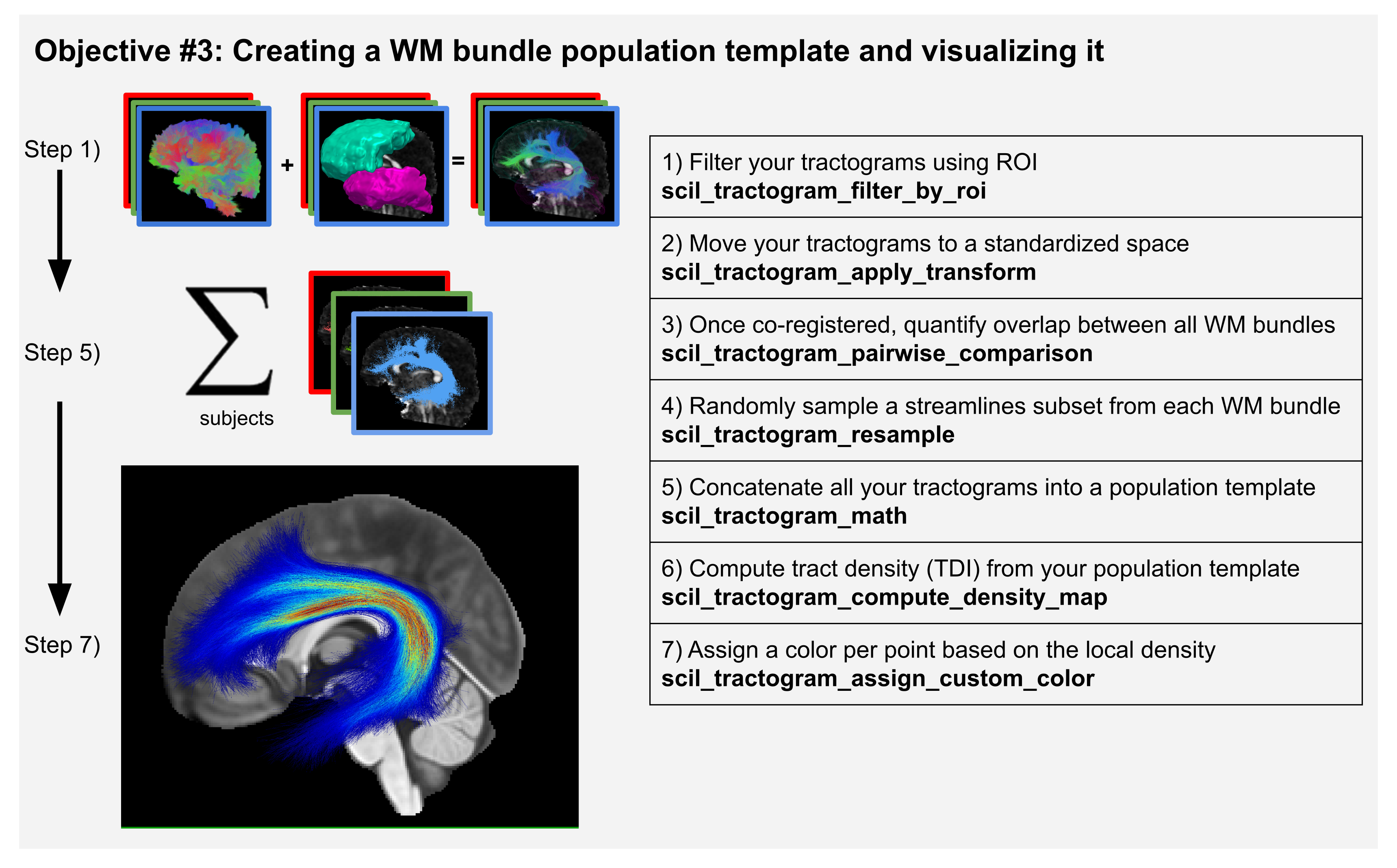
Scilpy scripts enable users to create a WM bundle population template, such as described in figure 3 in our upcoming paper. Such a pipeline includes:
segmenting the bundle of interest in each subject’s tractogram. The segmentation of bundles can be based on ROIs of inclusion / exclusion (scil_tractogram_segment_with_ROI_and_score or scil_tractogram_filter_by_roi) or based on the general shape of the streamlines (scil_tractogram_segment_with_recobundles, scil_tractogram_segment_with_bundleseg). See Tractogram Segmentation into bundles for more information on this.
registering the bundles to a reference space (e.g., MNI space) and analysing the inter-subject variability,
combining them into a reference bundle template, similarly to how one would average many structural MRI images to create a brain template.
analysing the results.
Then, registration can be performed (see Tractogram registration). The tractograms can be downsampled and concatenated (see Tractogram manipulations: logical operations, resampling, filtering) and even concatenated to their flipped version to obtain a symmetrical template.
Preparing data for this tutorial
To download data for this tutorial, see page Getting ready for tutorials. Then do:
MNI=$in_dir/mni_masked.nii.gz

# Current wmparc is in float. Should be in int. Let's convert.
scil_volume_math convert $in_dir/sub-01/sub-01__wmparc.nii.gz \
    --data_type int16  -f $in_dir/sub-01/sub-01__wmparc.nii.gz
The labels come from a Freesurfer segmentation, and the labels that it contains are found in the FsWiki’s Color Look-up Table (LUT) .
Tip
You may download the complete bash script to run the whole tutorial in one step ⭳ here.
Step A. Prepare the bundle of interest in each subject
for subj in "sub-01" # "sub-02" ... If we have many subjects, we can loop on each one
 do
     mkdir $subj
     echo "----> Processing subject $subj"

     # 1) Use any tool as you want to obtain a gray matter (GM) segmentation of
     #    your volume. Ex: Freesurfer. Here we already have wmparc.nii.gz.

     # 2) Split your volume into binary masks associated to each label.
     scil_labels_split_volume_by_ids $in_dir/$subj/${subj}__wmparc.nii.gz \
         --out_dir $subj/labels/ -v

     # 3) Segment the bundle using labels 2024 (ctx-rh-precentral) and 16 (Brain-Stem).
     #    The command below keeps all streamlines with at least one endpoint inside
     #    label 2024 and one endpoint inside label 16. This should select a CST bundle.
     #    The last numbers (3 and 2) are the maximum distance accepted for a endpoint
     #    to be considered inside the ROI.
     in_tractogram=$in_dir/$subj/${subj}_local_tractogram.trk
     out_tractogram=$subj/CST.tck
     scil_tractogram_filter_by_roi $in_tractogram $out_tractogram \
         --drawn_roi $subj/labels/2024.nii.gz either_end include 3 \
         --drawn_roi $subj/labels/16.nii.gz either_end include 2 -v

     # 4) Register to MNI space.
     #    You can use any tool for this, such as ANTs
     #    Here is how *we* created the transformation files.
     #    You need to have ANTs installed to run this:
     # mkdir $in_dir/$subj/transfo/
     # antsRegistrationSyNQuick.sh -d 3 -m $MNI \
     #     -f $in_dir/$subj/${subj}__fa.nii.gz -t r \
     #     -o $in_dir/$subj/transfo/MNI_ -n 4
     transfo=$in_dir/$subj/transfo/MNI_0GenericAffine.mat

     # 5) Apply the transformation to your tractogram.
     #    Uses the ANTs transformation. We used linear registration so we
     #    can use the .mat output.
     in_bundle=$subj/CST.tck
     out_bundle=$subj/CST_MNI.tck
     ref=$in_dir/$subj/${subj}__fa.nii.gz
     scil_tractogram_apply_transform $in_bundle $MNI $transfo $out_bundle \
         --inverse --cut_invalid --reference $ref

     # 6) (optional) You could subsampled subsets of streamlines
     in_bundle=$subj/CST_MNI.tck
     out_bundle=$subj/CST_MNI_resampled1000.tck
     scil_tractogram_resample $in_bundle 1000 $out_bundle \
         --never_upsample --reference $MNI
 done
Step B. Quantify inter-subject variability
We may quantify the overlap between all bundles across subjects.
scil_bundle_pairwise_comparison $out_dir/*/CST_MNI.tck \
        $out_dir/cst_stats.json --reference $MNI
Step C. Combine all subjects into a population template
Let’s combine all streamlines from all subjects and visualize the result.
# 1) Merge all CST files from all subjects together
scil_tractogram_math union $out_dir/*/CST_MNI_resampled1000.tck \
    $out_dir/merged_CST_MNI.tck --reference $MNI

# 2) Compute the density map
scil_tractogram_compute_density_map $out_dir/merged_CST_MNI.tck \
    $out_dir/merged_CST_MNI_density.nii.gz --reference $MNI

# 3) We color the streamlines with the values of the density map to create
#    the figure shown in step 7 of the figure.
scil_tractogram_assign_custom_color $out_dir/merged_CST_MNI.tck \
    $out_dir/merged_CST_MNI.tck --reference $MNI -f \
    --from_anatomy $out_dir/merged_CST_MNI_density.nii.gz